Scale-Space Blob Detection

Implementing a Laplacian blob detector in python from scratch

Features generated from Harris Corner Detector are not invariant to scale. For feature tracking, we need features which are invariant to affine transformations. Laplacian blob detector is one of the basic methods which generates features that are invariant to scaling.

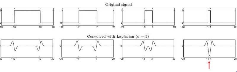
The idea of a Laplacian blob detector is to convolve the image with a “blob filter” at multiple scales and look for extrema of filter response in the resulting scale space.

Blob Filter:

This filter generated by double derivating Gaussian filter along x and y-axis and adding them. Above is also known as Laplacian of Gaussian.

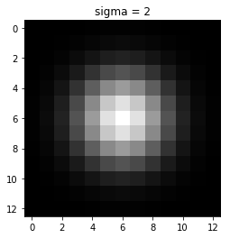
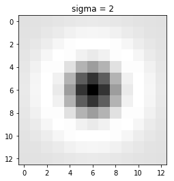
The output of the LOG filter is maximum when there is a corner in an image.

We want to find the characteristic scale of the blob, by convolving the image with different sigmas. But as we increase the sigma the response of blob filter with image decreases due to which we might not able to find a better scale. To reduce this effect we multiply the LOG filter σ square. This process is known as scale normalization.

The Laplacian archives maximum response for the binary circle of radius r is at σ=1.414*r

Above are some of the basics of the blob filter. The whole process boils down to two steps

1. Convolve image with scale-normalized Laplacian at several scales (different scales means different sigma)
2. Find maxima of squared Laplacian response in scale-space

Code for Laplacian Blob Detection

The code has four main steps:

1. Generation of LOG filters
2. Convolving the images with Gaussian filters
3. Finding the maximum peak
4. Drawing the blobs.

Generation of LOG filter

import cv2
from pylab import *
import numpy as np
import matplotlib.pyplot as plt
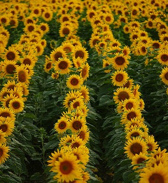
img = cv2.imread("sunflowers.jpg",0) #gray scale conversion
from scipy import ndimage
from scipy.ndimage import filters
from scipy import spatial
k = 1.414
sigma = 1.0
img = img/255.0  #image normalization

def LoG(sigma):
    #window size 
    n = np.ceil(sigma*6)
    y,x = np.ogrid[-n//2:n//2+1,-n//2:n//2+1]
    y_filter = np.exp(-(y*y/(2.*sigma*sigma)))
    x_filter = np.exp(-(x*x/(2.*sigma*sigma)))
    final_filter = (-(2*sigma**2) + (x*x + y*y) ) *  (x_filter*y_filter) * (1/(2*np.pi*sigma**4))
    return final_filter

LoG function takes sigma as input and generates a filter of size 6*sigma(best option).

Convolving the images with Gaussian filters

The images are convolved with different LOG filters

def LoG_convolve(img):
    log_images = [] #to store responses
    for i in range(0,9):
        y = np.power(k,i) 
        sigma_1 = sigma*y #sigma 
        filter_log = LoG(sigma_1) #filter generation
        image = cv2.filter2D(img,-1,filter_log) # convolving image
        image = np.pad(image,((1,1),(1,1)),'constant') #padding 
        image = np.square(image) # squaring the response
        log_images.append(image)
    log_image_np = np.array([i for i in log_images]) # storing the #in numpy array
    return log_image_np
log_image_np = LoG_convolve(img)
#print(log_image_np.shape)

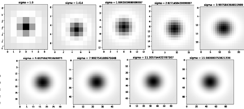
To choose different sigma, I have multiplied sigma with k^i.The dimension of the log_image_np array will be z*image_height*image_width.where z represents the kth power that is multiplied to sigma.

In the above function, I have generated only 9 filters the plot of 9 filters are

Finding the maximum peak

def detect_blob(log_image_np):
    co_ordinates = [] #to store co ordinates
    (h,w) = img.shape
    for i in range(1,h):
        for j in range(1,w):
            slice_img = log_image_np[:,i-1:i+2,j-1:j+2] #9*3*3 slice
            result = np.amax(slice_img) #finding maximum
            if result >= 0.03: #threshold
                z,x,y = np.unravel_index(slice_img.argmax(),slice_img.shape)
                co_ordinates.append((i+x-1,j+y-1,k**z*sigma)) #finding co-rdinates
    return co_ordinates
co_ordinates = list(set(detect_blob(log_image_np)))

At each pixel 3×3 neighborhood is considered in all scales which gives the 9x3x3 matrix. The maximum peak of the matrix is given by the maximum value of the matrix.

For every pixel, there will be a maximum. But not all pixels contribute to blobs. So we need to eliminate them by thresholding the peaks. This threshold is found by trial and error method.

If the maximum value is greater than the threshold then the point is considered and coordinate is stored.

(z,x,y) is the coordinates of the sliced image so we need to change them to original image coordinates. After changing them we will store them in the co_ordinates list and plot them.

fig, ax = plt.subplots()
nh,nw = img.shape
count = 0

ax.imshow(img, interpolation='nearest',cmap="gray")
for blob in co_ordinates:
    y,x,r = blob
    c = plt.Circle((x, y), r*1.414, color='red', linewidth=1.5, fill=False)
    ax.add_patch(c)
ax.plot()  
plt.show()

The above code draws the blob at each point in the stored list.

Result

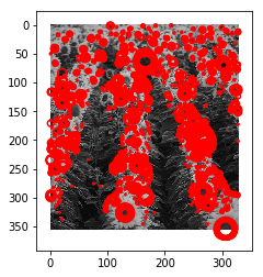
In the above image, we can find many blobs are overlapping. To reduce overlapped blobs we will find the area of overlap between blobs. If the area is greater than the threshold the blob with the smaller radius will be discarded.

#provided in scipy doucumentaion
def blob_overlap(blob1, blob2):
    n_dim = len(blob1) - 1
    root_ndim = sqrt(n_dim)
    #print(n_dim)
    
    # radius of two blobs
    r1 = blob1[-1] * root_ndim
    r2 = blob2[-1] * root_ndim
    
    d = sqrt(np.sum((blob1[:-1] - blob2[:-1])**2))
    
    #no overlap between two blobs
    if d > r1 + r2:
        return 0
    # one blob is inside the other, the smaller blob must die
    elif d <= abs(r1 - r2):
        return 1
    else:
        #computing the area of overlap between blobs
        ratio1 = (d ** 2 + r1 ** 2 - r2 ** 2) / (2 * d * r1)
        ratio1 = np.clip(ratio1, -1, 1)
        acos1 = math.acos(ratio1)

ratio2 = (d ** 2 + r2 ** 2 - r1 ** 2) / (2 * d * r2)
        ratio2 = np.clip(ratio2, -1, 1)
        acos2 = math.acos(ratio2)

a = -d + r2 + r1
        b = d - r2 + r1
        c = d + r2 - r1
        d = d + r2 + r1

area = (r1 ** 2 * acos1 + r2 ** 2 * acos2 -0.5 * sqrt(abs(a * b * c * d)))
        return area/(math.pi * (min(r1, r2) ** 2))
    
def redundancy(blobs_array, overlap):
    sigma = blobs_array[:, -1].max()
    distance = 2 * sigma * sqrt(blobs_array.shape[1] - 1)
    tree = spatial.cKDTree(blobs_array[:, :-1])
    pairs = np.array(list(tree.query_pairs(distance)))
    if len(pairs) == 0:
        return blobs_array
    else:
        for (i, j) in pairs:
            blob1, blob2 = blobs_array[i], blobs_array[j]
            if blob_overlap(blob1, blob2) > overlap:
                if blob1[-1] > blob2[-1]:
                    blob2[-1] = 0
                else:
                    blob1[-1] = 0

return np.array([b for b in blobs_array if b[-1] > 0])

co_ordinates = np.array(co_ordinates)
co_ordinates = redundancy(co_ordinates,0.5)

After removing overlapped blobs the output is

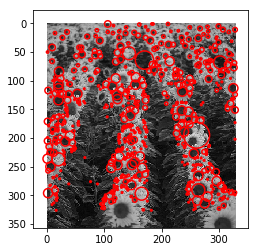
We can see that most of the blobs have been eliminated.

Link for the code in Github.

Thanks for reading. Any suggestions would be appreciated.