Face Recognition and Neural Style Transfer in Deep Learning
Face Recognition:
Before looking into what face recognition is and how it works, let us understand the difference between face recognition and face verification.
Face Verification checks “is this the claimed person?”. For example, in school, you go with your ID card and the invigilator verifies your face with the ID card. This is Face Verification. A mobile phone that unlocks using our face is also using face verification. It is 1:1 matching problem.
Now suppose the invigilator knows everyone by their name. So, you decide to go there without an ID card. The invigilator identifies your face and let you in. This is Face Recognition. Face Recognition deals with “who is this person?” problem. We can say that it is a 1:K problem.
Before starting with face recognition let us look into how we solve the problem of face verification.
Pixel-by-Pixel Comparison:
A naïve method to perform face verification is pixel-by-pixel comparison. If the distance between both the images is less than a certain threshold value then they are of the same person or not.

But this algorithm performs poorly, since the pixel values in an image change dramatically even with a slight change of light, position or orientation. In this case, the face embeddings come to rescue. You’ll see that rather than using the raw image, you can learn an encoding f(img) so that element-wise comparisons of this encoding gives more accurate judgements as to whether two pictures are of the same person.
Now we can list out the steps involved in Face recognition (using face verification):
⦁ Create embeddings of the images,
⦁ Using the Siamese networks (one-shot learning) perform face verification
⦁ Using Triplet Loss (formalization of face verification), train the model to perform the task of face recognition.
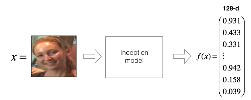
Embeddings:
Embeddings or encodings are a 128-dimensional vectoral representation of a given image.
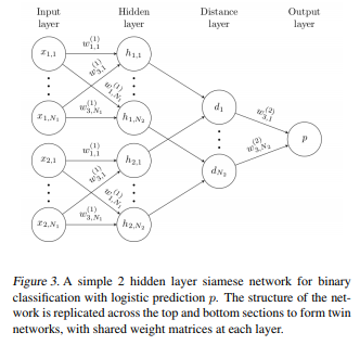
Siamese Networks (One-shot Learning):
Siamese Networks are two identical networks with shared weights and parameters. Instead of directly classifying an input(test) image to one of the 10 people in the organization, this network instead takes an extra reference image of the person as input and will produce a similarity score denoting the chances that the two input images belong to the same person. Typically the similarity score is squished between 0 and 1 using a sigmoid function; wherein 0 denotes no similarity and 1 denotes full similarity. Any number between 0 and 1 is interpreted accordingly.
Notice that this network is not learning to classify an image directly to any of the output classes. Rather, it is learning a similarity function, which takes two images as input and expresses how similar they are.
The main intuition behind these networks is that if two images are similar the element wise difference between their embeddings is also small. Similarly, for different images, the difference between the embeddings is high and hence the score given by these networks is also high.
Triplet Loss:
Training will use triplets of images :
⦁ A is an “Anchor” image–a picture of a person.
⦁ P is a “Positive” image–a picture of the same person as the Anchor image.
⦁ N is a “Negative” image–a picture of a different person than the Anchor image.
These triplets are picked from our training dataset. We will write (A(i),P(i),N(i)) to denote the i-the training example.
You’d like to make sure that an image of an individual is closer to the Positive than to the Negative image by at least a margin α.
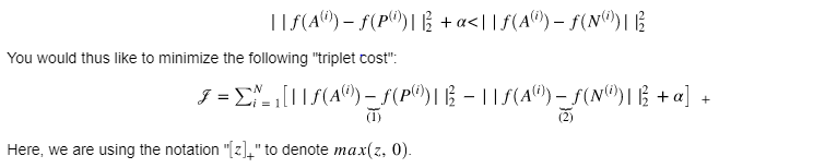
Notes:
⦁ The term (1) is the squared distance between the anchor “A” and the positive “P” for a given triplet; you want this to be small.
⦁ The term (2) is the squared distance between the anchor “A” and the negative “N” for a given triplet, you want this to be relatively large, so it thus makes sense to have a minus sign preceding it.
⦁ α is called the margin. It is a hyperparameter that you should pick manually. We will use α=0.2.
Now triplet loss can be used to train a model which performs face verification. To perform face recognition given an image we can perform face verification to every image in the database and obtain the score. As already stated Face recognition is a 1:K problem where a single image is compared to K images.
Check our article on DeepFace and Facenet for face recognition for more details about face recognition.
Neural Style Transfer:
Neural style transfer is an optimization technique that merges content (C), style image(S) to create a generated image(G). The input image is transformed to look like the content image, but “painted” in the style of the style image

Generally, the VGG19 architecture is used to achieve this task. We need to choose a certain layer whose activation we will be taking for the content or the style. The shallow layers of any NN tend to detect lower-level features such as edges and simple textures, and the later (deeper) layers tend to detect higher-level features such as more complex textures as well as object classes. Thus, somewhere between where the raw image is fed in and the classification label is output, the model serves as a complex feature extractor; hence by accessing intermediate layers, we’re able to describe the content and style of input images.
There are three steps involved in NST.
⦁ Compute the content Cost Function Jcontent(C,G)
⦁ Compute the Style Cost Function Jstyle(S,G)
⦁ Combine these to obtain the overall cost function J(G)
⦁ Content Cost Function:
Let a(C) be the activation of the hidden layer which gives the content information. It is of dimension nHnWnc. Same is tha case for a(G). The content Loss is
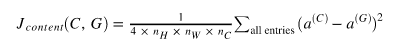
To compute the difference the 3D activations are unrolled to 2D as shown in the figure.

⦁ Style Cost Function:
Style matrix or Gram Matrix:
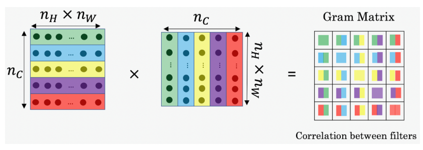
To obtain the style matrix the activation of the style image is multiplied with its transpose. The result is a matrix of dimension (nc * nc). The value Gi j measures how similar the activations of filter i are to the activations of filter j.
Style Cost:
Our goal is to minimize the distance between gram matrix of the style image(S) and that of the generated image (G).

This style function is computed across various layers (Considering activations at various levels).
⦁ Total Cost Function:
The total cost function is defined as
J(G) = α Jcontent(C,G)+β Jstyle(S,G)


1 Comment
DeepFace and Facenet for face recognition - projectsflix · July 20, 2019 at 11:38 am
[…] Check our article for more methods on Face recognition. […]